Smooth Refraction Approximation Layered Model (SRAL)
This is a part of the blog post series Rendering Layered Materials.
Here I present my approach to the layered surface material as an alternative to the layered model by Andrea Weidlich and Alexander Wilkie from 2007 (which I refer to as the WWL model or just the original model). This part contains an overall explanation of my model, its evaluation and sampling process, and a few example result images.
Overall model description
At first sight, my layered model doesn’t differ very much from the WWL model, but it contains important improvements, which solve several problems of the previous model and offers a rigorous formulation of the model built upon the radiometry and the Monte Carlo integration framework. Namely, the improvements are:
- Using geometric normal for refraction instead of the reflection micro-facet’s one.
- Adding the missing compensation of solid angle (de-)compression effects in both evaluation and sampling – solves the energy conservation problem and incorrect sampling PDF leading to a biased Monte-Carlo estimator.
- Properly designed and more efficient sampling strategy.
The model has two main parameters – two stand-alone layer BSDFs, which I denote
where index 1 means outer layer, index 2 means inner layer, $x$ is the surface point at which the model is evaluated, $\omega_{i}$ is the incident light direction, and $\omega_{o}$ is the outgoing light direction. For the sake of clarity, I will, from time to time, omit some of the parameters. Any direction $\omega$ can be expressed as a pair of angles $\left(\phi,\theta\right)$, where $\phi$ is the azimuth and $\theta$ is the inclination, i.e. angle between the direction and the surface normal.
The resulting model BSDF $f_{s}$ can be understood as a sum of two sub-BSDFs $f_{s1}^{\ast}$ and $f_{s2}^{\ast}$ representing the contributions of the respective layers, which I sometimes call contribution BSDFs or layers’ contributions:
The outer layer is assumed to be a micro-facet-based interface between two media with refractive indices $\eta_0$ and $\eta_1$. The inner layer is assumed to be reflection only, i.e. without transmission component. There is no assumption on the medium below the inner layer.
Refraction through the geometrical normal
The new model still assumes single-point simplifications of both evaluation and sampling used in the original model, as well as non-scattering medium between layers. However, unlike the WWL model, it doesn’t make any assumption about the relative size of micro-facets and layers, which served as a justification for using the reflection-defined micro-facet normal during the evaluation and sampling process. For computing refractions, my model uses the geometrical normal rather than the micro-facet’s one. The result is that it behaves as if the light refracted through a virtual ideally smooth surface instead of through the arbitrarily rough micro-facet outer layer. This way the same amount of energy gets refracted, but in a single direction instead of through a set of directions. Obviously, the higher the specularity of the outer surface is the better this approximation behaves.

The new model still estimates the whole sub-surface light transport with just one light path and a single scattering event, but the used refraction directions define a path, which is more likely the one through which the peak amount of energy flows.
It is good to keep in mind that both models neglect the energy which is reflected from the inside of the outer layer back into the medium and reemerges on the surface after multiple scattering events between the layers. The WWL model uses some kind of compensation for the missing energy, but the paper doesn’t explain this in detail.
Evaluation
As mentioned earlier, the model can be understood as a sum of two contribution BSDFs:
Outer layer
The contribution BSDF of the outer layer is rather trivial. The incident light is partially reflected and partially refracted. The light which gets refracted through the first layer is accounted for within the inner layer component so we ignore it here and the renderer must make sure that it is not evaluated for directions below surface. Since the reflected light is unaffected by the rest of the model and the whole model takes only reflection directions into account, it can be evaluated directly by evaluating the outer layer BSDF $f_{s1}$ without any modification:
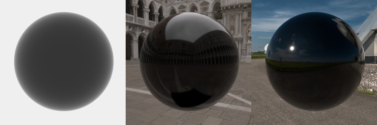
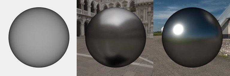
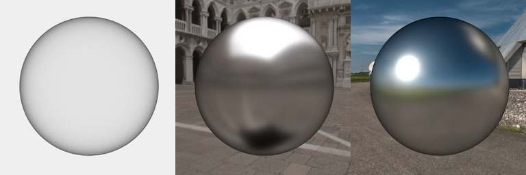
Reflection contribution of a highly glossy micro-facet outer layer (Smith micro-surface profile, GGX distribution with roughness 0.01, air-glass interface) under various light settings (constant light, large light source, small light source).
Inner layer
For the inner layer, the things are considerably more complicated because the light which reaches it undergoes refraction when passing the outer layer, gets attenuated by the medium between the layers, and gets refracted again when passing the model through the outer layer for the second time. Let’s have a look at how do these mechanisms affect the inner layer contribution one after another.
Naïve refraction
Let’s start with an inner layer (Lambert in the example picture) without any modifications, which will undergo the aforementioned modifications later on:

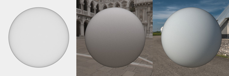
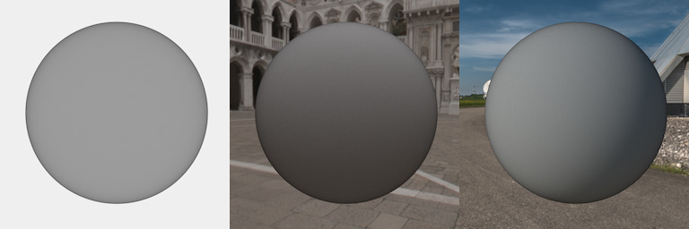
Plain, ideally white Lambert without any modifications under various light settings.
The inner layer is evaluated for refracted directions $\omega_{i}^{\prime}$ and $\omega_{o}^{\prime}$ instead of the directions at the outer layer $\omega_{i}$ and $\omega_{o}$. After replacing the directions, the inner layer contribution will look like this:

Ideally white Lambert with refracted directions under various light settings. Since Lambert model is a constant BSDF, changing directions doesn't change the shape of the BSDF in the upper hemisphere; therefore, the behaviour is identical to the version with unmodified directions. Behaviour of non-constant inner layers with refracted parameters will be shown later.
The light passing through the smooth interface gets attenuated according to the Fresnel equations:
Where $T\left(\theta_{i}\right)$ and $T\left(\theta_{o}\right)$ are the Fresnel transmission coefficients.
Ideally white Lambert with refracted directions and Fresnel attenuation under various light settings. Fresnel components affects the amount of transmitted light mostly at grazing angles.
Medium attenuation
After refraction, we add the effect of medium attenuation. In a non-scattering medium, the attenuation $a$ can be well modeled with the Beer-Lambert-Bouguer law, exactly as it was done in the original paper:
where $\alpha$ is the medium attenuation coefficient, $d$ is the thickness of the layer, and $\theta_{i}^{\prime}$ and $\theta_{o}^{\prime}$ are inclinations of the respective refraction directions. The BSDF is now
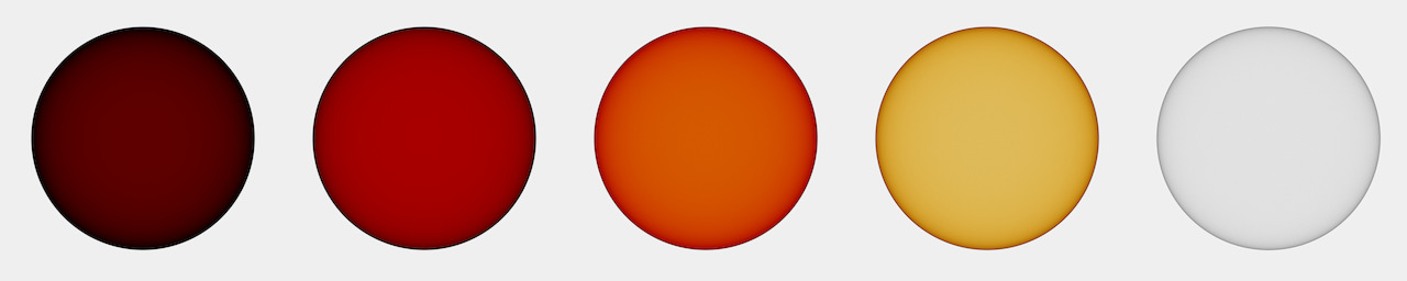
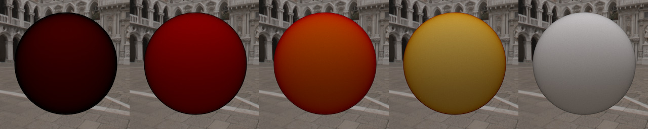
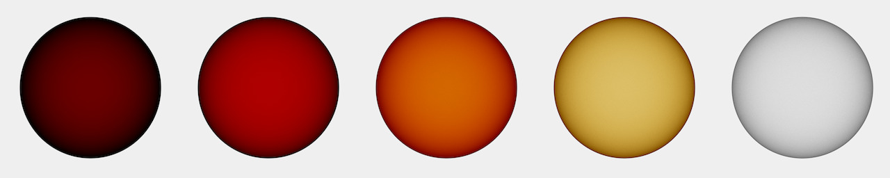
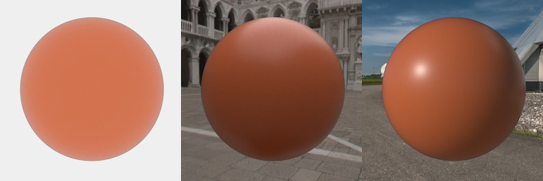
Ideally white Lambert layer with refracted directions, Fresnel attenuation and orange medium attenuation with several medium thicknesses under various light settings. You can nicely see the effect of darkening and colour saturation when the light passed through thicker layers.
Proper refraction
Although everything looks pretty straightforward in the previous images, a problem arises if we use a non-constant BSDF for the inner layer:

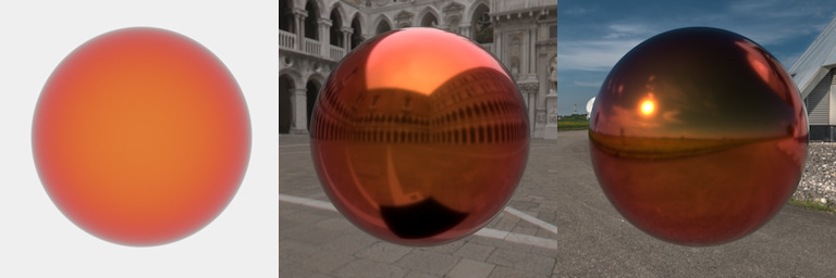
Broken energy conservation due to refracted directions: Glossy inner layer (GGX roughness 0.1) with refracted directions, Fresnel attenuation under orange medium with varying medium thickness under constant lighting.
Although we used a physically-plausible energy-conserving model for the inner layer, the resulting inner layer model is in some scenarios much lighter than one would expect. In the furnace test (constant white light configuration) we can clearly see that it reflects more energy than it receives from the environment which is a sign of an energy conservation problem. I spent a non-trivial amount of time to crack this problem, but I won in the end and I gained some important computer graphics knowledge on this way. Long story short: the problem is caused by ignoring the compression and decompression of light when crossing an interface between media with different indices of refraction.
I derived a correct energy-conserving BSDF under a smooth refractive interface with a single scattering event. For that I dug deeper into the theory of BDSFs in another post called Energy Conserving BSDF Under a Smooth Refractive Interface. If you are not feeling nerdy enough, just ignore it :-) – it basically says that the thing our original naïve refraction approach is missing is the (relatively trivial) compensation factor $\frac{\eta_{0}^{2}}{\eta_{1}^{2}}$, which, however, makes the difference:
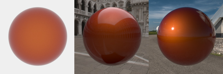
Energy conservation fixed with solid angle compression compensation $\frac{\eta_{0}^{2}}{\eta_{1}^{2}}$: Glossy inner layer (GGX roughness 0.1) with refracted directions, Fresnel attenuation under orange medium with varying medium thickness under constant lighting.
The result may now, in fact, look much darker than expected for some settings (especially for highly diffuse models like Lambert), but it is caused by the single scattering nature of our model, which neglects the energy which is reflected from the outer layer from the inside back to the medium:
Darkening due to missing multi-scattered energy. Ideally white Lambert inner layer with refracted directions under various light settings.
In case of ideally diffuse (constant) inner layer, one can partially compensate the missing multi-scattered energy by omitting the compensation factor $\frac{\eta_{0}^{2}}{\eta_{1}^{2}}$. This will put back into equation the energy which gets reflected back to the medium through total internal reflection (TIR), but not the energy which undergoes partial reflection. This basically leads to the results of the “naïve refraction” approach:
Compensation of the missing in-scattered energy due to TIR for a ideally diffuse inner layer by omitting the solid angle (de-)compression compensation factor $\frac{\eta_{0}^{2}}{\eta_{1}^{2}}$.
Unfortunately, this approach is not applicable in case of non-diffuse inner layers.
Inner layer formula
If we put together all the components which affect the inner layer contribution, we’ll get the final formula for the inner layer contribution:
where $f_{s2}\left(\omega_{i}^{\prime}\rightarrow\omega_{o}^{\prime}\right)$ is the stand-alone BSDF of the inner layer, $T\left(\theta_{i}\right)$ and $T\left(\theta_{o}\right)$ are the Fresnel transmission coefficients, $\frac{\eta_{0}^{2}}{\eta_{1}^{2}}$ is the projected solid angle compression compensation and $a$ is the medium attenuation coefficient.
Just a side note: Since we are implicitly assume a rendering system which is not polarization aware, we don’t have to worry about the order in which the coefficients are multiplied together. In a polarization-aware system, however, multiplication operations (representing light-matter interaction) have to be dealt with much more care.
Whole formula
To summarize, the complete BSDF formula containing contributions of both layers is
where $f_{s1}$ and $f_{s2}$ are the stand-alone outer and inner layer BSDFs, $T \left(\theta_{i}\right)$ and $T\left(\theta_{o}\right)$ are the Fresnel transmission coefficients, $a\left(\theta_{i}, \theta_{o}\right)$ is the medium attenuation (see section “Medium attenuation” for details) and $\frac{\eta_{0}^{2}}{\eta_{1}^{2}}$ is the projected solid angle (de-)compression compensation. It’s important to note that the formula is, in fact, just a BRDF rather than a BSDF, because it is properly defined only for directions from the upper hemisphere.
The complete model for glossy outer layer may look like this (more examples at the end of the post):

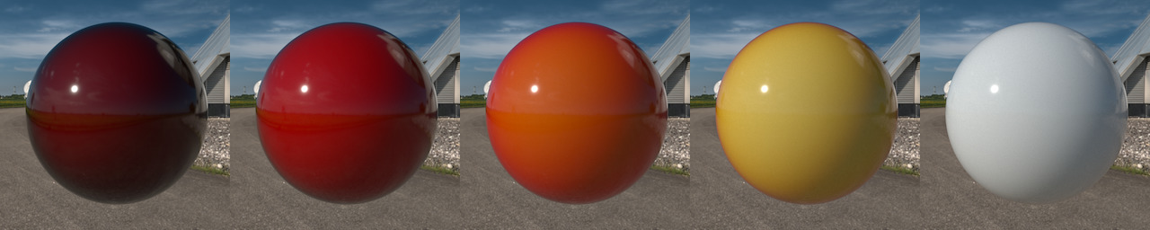
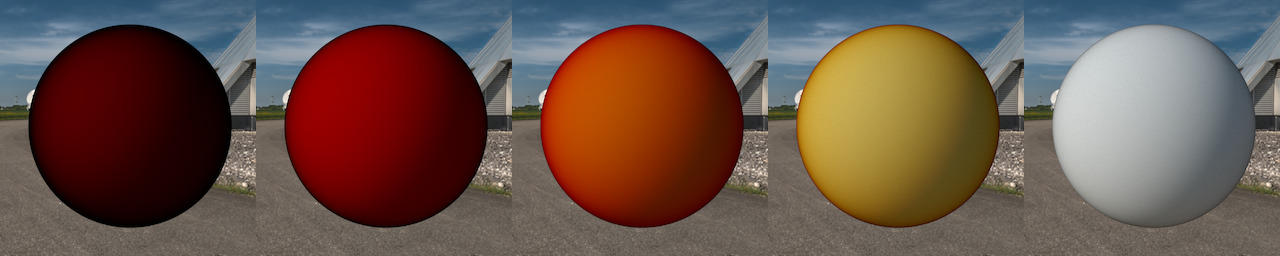
The whole formula using almost specular outer layer, ideally white Lambert inner layer and orange medium between them with varying medium thickness under various light settings. Compensation of the missing in-scattered energy due to TIR by omitting the solid angle (de-)compression compensation is applied.

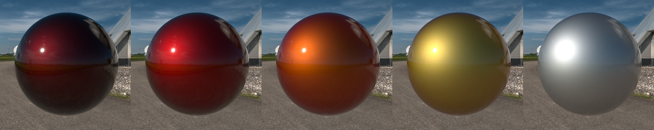
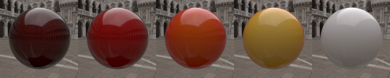
The whole formula using almost specular outer layer, glossy conductor inner layer and orange medium between them with varying medium thickness under various light settings.
Sampling
In a Monte Carlo-based (MC) rendering system (e.g. path tracing) a BSDF model needs to provide not only its evaluation formula, but also a direction sampling strategy with evaluation of its PDF. To denote a sampling strategy it is often sufficient to use the symbol of its PDF (e.g. $p$).
In our layered model we assume that the stand-alone outer and inner layer BSDFs $f_{s1}$ and $f_{s2}$ provide their own reasonably efficient sampling strategies $p_1$ and $p_2$ respectively, which we will use to build a sampling strategy for the whole model. Since our BSDF is a simple sum of two slightly modified BSDFs, we can build a reasonably efficient overall sampling strategy $p$ by simple blending of their slightly modified strategies:
where $p_1^{\ast}$ and $p_2^{\ast}$ are modified sampling strategies of the respective BSDF layers contributions, $\omega_{i}$ is the (sampled) direction of incident light, $\omega_{o}$ is the (fixed) outgoing light direction and $w_1$ and $w_2$ are some blending coefficients.
First, we’ll have a look at separate sampling strategies $p_1^{\ast}$ and $p_2^{\ast}$, then we’ll combine them together to obtain $p$.
Outer layer sampling
Because the outer layer BSDF $f_{s1}$ is evaluated directly without any modification, we can use the original sampling strategy of the outer layer stand-alone BSDF
The renderer just has to instruct the sampling routine to draw samples only from the upper hemisphere because we are interested only in the reflected contribution of the layer, not refracted.
Inner layer sampling

Sampling geometry for the inner layer contribution component, where $f_{s1}$ is the smooth interface, $f_{s2}$ is the inner layer BSDF.
Sampling the inner layer component is not hard either, although a little bit tricky. We have to feed the original strategy of the inner stand-alone BSDF with the refracted version of the outgoing direction and refract the generated incoming direction through the virtual smooth interface back into the outside world. This approach will modify the shape of the original sampling PDF in the same way we modified the shape of the original stand-alone BSDF.
It is possible that the generated direction is refracted back into the model due to total internal reflection (TIR). The resulting sample in such case is valid, it must not be discarded and its contribution is zero because our model neglects energy which undergoes multiple scattering events.
Now that we have constructed the sampling routine, we also need to evaluate its PDF. At first sight it seems that we just have to evaluate the original PDF using the refracted directions $\omega_{i}^{\prime}$ and $\omega_{o}^{\prime}$, analogically to the way we modified the original sampling strategy
However, if we feed a MC renderer with such PDF, the result will look like this:
Too dark inner layer problem: Glossy conductor inner layer with refracted direction and Fresnel attenuation under various light settings.
As you can see, the result is much darker than it should be. The reason is that the change of directions due to refraction also changes the solid angular density of directional samples. Since the sampling PDF expresses the density of generated samples with respect to the solid angle measure, we need to compensate the original PDF accordingly to get the correct value.
This compensation factor is closely related to what happens to radiance when it gets refracted through a smooth interface between two media with different refractive indices. Its application will finally yield the correct PDF values resulting in an unbiased Monte Carlo estimator leading to the correct rendering output:
Too dark inner layer problem fixed: Glossy conductor inner layer with refracted direction and Fresnel attenuation under various light settings.
Sampling both layers
To obtain an efficient MC estimator of the rendering integral, the sampling PDF has to be as proportional to the integrand as possible. Ideally, the sampling PDF should be the normalized version of the integrand. i.e. scaled by a factor to make its integral over the whole sphere equal 1. The integrand in the practically used form is
However, because we usually don’t know the distribution of the incident radiance, the sampling routine is usually trying to mimic at least the product of the BSDF and the cosine factor
In the case of our layered model, the BSDF is a sum of two components so the integrand looks like
It would not be reasonable to try to derive a sampling strategy directly for the sum formula because its components are general functions which can be hard to sample even separately and which we have little information about anyway. We will instead build the overall sampling strategy on top of the already existing strategies $p_1^{\ast}$ and $p_2^{\ast}$ by blending them together.
If we can sample and evaluate both $p_1^{\ast}$ and $p_2^{\ast}$, it is easy to sample and evaluate a weighted average of the two
given that weights $w_1$ and $w_2$ are normalized (their sum equals 1). The question is how to choose the weights to make the resulting PDF as proportional to whole $f_{s}$ as possible. Ideally, the weights should be proportional to the integrals of respective components and the overall strategy would then be as good as the partial ones. The problem is that the integrals are in general hard to evaluate precisely so we have to resort to an approximation.
Outer layer integral
On the outer layer, the light is either reflected from or refracted through the layer’s micro-facets. We will approximate the amount of reflected light just by the Fresnel reflection coefficient of a smooth interface:
Inner layer integral
Let’s recall the inner layer contribution
therefore, we need to approximate its integral
Note that integral components independent from $\omega_{i}$ were moved outside the integral and we integrate only over the upper hemisphere $\mathcal{H}_{+}^{2}$ rather than over the whole sphere $\mathcal{S}^{2}$ because there’s no transmission through the inner layer allowed.
While the components outside the integral are easy to evaluate analytically, the integral part is more complicated and has to be approximated. We will start with the partial integral
We assume that the stand-alone BSDF $f_s$ can compute its reflectance over the upper hemisphere
and we will use it as a base approximation of the partial integral. This is rather inaccurate because $\rho_{s2}$ uses the original directions $\omega_{i}$ and $\omega_{o}$ instead of their refracted versions $\omega_{i}^{\prime}$ and $\omega_{o}^{\prime}$; therefore, the shape of the integrand is not stretched out and also contains the parts which are cut away by the total internal reflection in our model, which can lead to substantial error especially at grazing angles. However, this approximation contains – at least partially – the characteristics of the inner material and should be better than ignoring it completely.
Both missing components $T\left(\theta_{i}\right)$ and $a\left(\theta_{i}, \theta_{o}\right)$ change the shape of the integrand and have to be taken into account, but their effect is hard to solve analytically. One way to approximate their overall effect is to evaluate them over the mirror reflection path ($\theta_{i} = \theta_{o}$) – analogically to what we did in evaluating the sub-surface scattering contribution of the whole model – and pretend they are constant over the whole hemisphere.
After putting everything together, the resulting approximation for the inner layer contribution integral is
Where $\eta_{0}^{2}$ and $\eta_{1}^{2}$ are refractive indices of the respective media, $T\left(\theta_{o}\right)$ is the Fresnel transmission coefficient, $a\left(\theta_{i}, \theta_{o}\right)$ is the medium attenuation (see the section “Medium attenuation” for more details), and $\rho_{s2}$ is the reflectance of the stand-alone inner layer BSDF.
Complete sampling routine
Now that we have the integral approximations $w_{1}$ and $w_{2}$, we obtain the PDF weights by normalizing the approximations
which define our mighty overall sampling routine
To sample from blended PDF, we have to first randomly pick one of the sampling sub-routines $p_1^{\ast}$ and $p_2^{\ast}$ with probabilities equal to $w_1$ and $w_2$ respectively and then draw sample from the selected sub-routine. To evaluate the probability density of the sample, evaluate the whole PDF $p$.
Results
Example images of different types configurations (with names from the original paper):

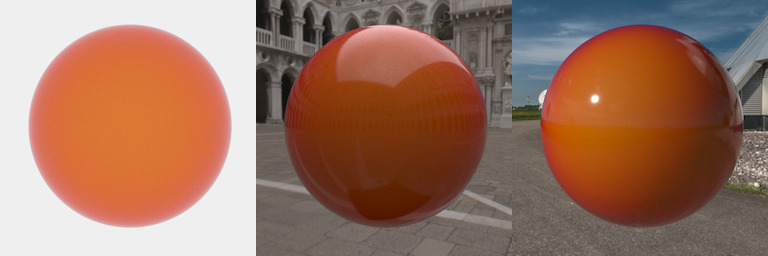
Glossy Paint: Orange Lambert inner layer, clear medium, and smooth outer layer. Compensation of missing TIR is applied.
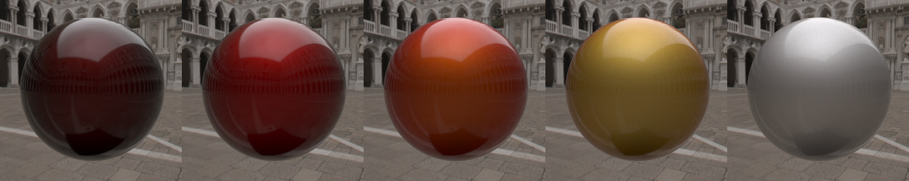
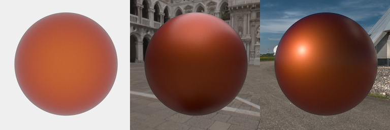
Frosted Paint: Orange Lambert inner layer, clear medium, glossy outer layer. Compensation of missing TIR is applied.
Metal Foil: Smooth inner layer, coloured medium, smooth outer layer.
Metallic Paint: Glossy inner layer, coloured medium, smooth outer layer.
Tinted Glazing: White Lambert inner layer, coloured medium, smooth outer layer. Compensation of missing TIR is applied.
Frosted Metal: Glossy inner layer, coloured medium, glossy outer layer.